py12box model usage

This notebook shows how to set up and run the AGAGE 12-box model.

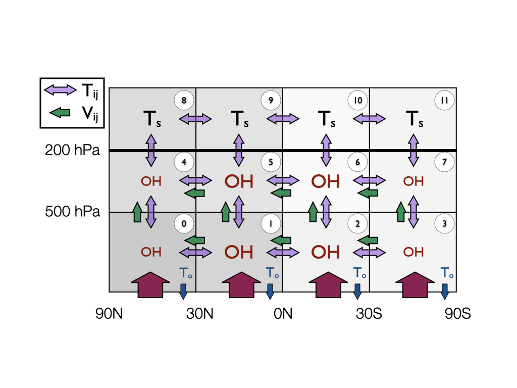
Model schematic

The model uses advection and diffusion parameters to mix gases between boxes. Box indices start at the northern-most box and are as shown in the following schematic:

Model inputs

We will be using some synthetic inputs for CFC-11. Input files are in:

data/example/CFC-11

The location of this folder will depend on where you’ve installed py12box and your system. Perhaps the easiest place to view the contents is in the repository.

In this folder, you will see two files:

CFC-11_emissions.csv

CFC-11_initial_conditions.csv

As the names suggest, these contain the emissions, initial conditions and lifetimes.

Emissions

The emissions file has four columns: year, box_1, box_2, box_3, box_4.

The number of rows in this file determines the length of the box model simulation.

The year column should contain a decimal date (e.g. 2000.5 for ~June 2000), and can be monthly or annual resolution.

The other columns specify the emissions in Gg/yr in each surface box.

Initial conditions

The initial conditions file can be used to specify the mole fraction in pmol/mol (~ppt) in each of the 12 boxes.

How to run

Firstly import the Model class. This class contains all the input variables (emissions, initial conditions, etc., and run functions).

We are also importing the get_data helper function, only needed for this tutorial, to point to input data files.

# Import from this package
from py12box.model import Model
from py12box import get_data

# Import matplotlib for some plots
import matplotlib.pyplot as plt

The Model class takes two arguments, species and project_directory. The latter is the location of the input files, here just redirecting to the “examples” folder.

The initialisation step may take a few seconds, mainly to compile the model.

# Initialise the model
mod = Model("CFC-11", get_data("example/CFC-11"))

Compiling model and tuning lifetime...
... completed in 3 iterations
... stratospheric lifetime: 52.1
... OH lifetime: 1e12
... ocean lifetime: 1e12
... non-OH tropospheric lifetime: 1e12
... overall lifetime: 52.0
... done in 5.5602850914001465 s

Assuming this has compiled correctly, you can now check the model inputs by accessing elements of the model class. E.g. to see the emissions:

mod.emissions

array([[100,  10,   0,   0],
       [100,  10,   0,   0],
       [100,  10,   0,   0],
       ...,
       [  0,   0,   0,   0],
       [  0,   0,   0,   0],
       [  0,   0,   0,   0]])

In this case, the emissions should be a 4 x 12*n_years numpy array. If annual emissions were specified in the inputs, the annual mean emissions are repeated each month.

We can now run the model using:

# Run model
mod.run()

... done in 0.024969100952148438 s

The primary outputs that you’ll be interested in are mf for the mole fraction (pmol/mol) in each of the 12 boxes at each timestep.

Let’s plot this up:

plt.plot(mod.time, mod.mf[:, 0])
plt.plot(mod.time, mod.mf[:, 3])
plt.ylabel("%s (pmol mol$^{-1}$)" % mod.species)
plt.xlabel("Year")
plt.show()

We can also view other outputs such as the burden and loss. Losses are contained in a dictionary, with keys: - OH (tropospheric OH losses) - Cl (losses via tropospheric chlorine) - other (all other first order losses)

For CFC-11, the losses are primarily in the stratosphere, so are contained in other:

plt.plot(mod.emissions.sum(axis = 1).cumsum())
plt.plot(mod.burden.sum(axis = 1))
plt.plot(mod.losses["other"].sum(axis = 1).cumsum())

[<matplotlib.lines.Line2D at 0x7f7824f23070>]

Another useful output is the lifetime. This is broken down in a variety of ways. Here we’ll plot the global lifetime:

plt.plot(mod.instantaneous_lifetimes["global_total"])
plt.ylabel("Global instantaneous lifetime (years)")

Text(0, 0.5, 'Global instantaneous lifetime (years)')

Setting up your own model run

To create your own project, create a project folder (can be anywhere on your filesystem). The folder must contain two files:

<species>_emissions.csv

<species>_initial_conditions.csv

To point to the new project, py12box will expect a pathlib.Path object, so make sure you import this first:

from pathlib import Path
new_model = Model("<SPECIES>", Path("path/to/project/folder"))

Once set up, you can run the model using:

new_model.run()

Note that you can modify any of the model inputs in memory by modifying the model class. E.g. to see what happens when you double the emissions:

new_model.emissions *= 2.
new_model.run()

Changing lifetimes

If no user-defined lifetimes are passed to the model, it will use the values in data/inputs/species_info.csv

However, you can start the model up with non-standard lifetimes using the following arguments to the Model class (all in years):

lifetime_strat: stratospheric lifetime

lifetime_ocean: lifetime with respect to ocean uptake

lifetime_trop: non-OH losses in the troposphere

e.g.:

new_model = Model("<SPECIES>", Path("path/to/project/folder"), lifetime_strat=100.)

To change the tropospheric OH lifetime, you need to modify the oh_a or oh_er attributes of the Model class.

To re-tune the lifetime of the model in-memory, you can use the tune_lifetime method of the Model class:

new_model.tune_lifetime(lifetime_strat=50., lifetime_ocean=1e12, lifetime_trop=1e12)